 开萌笔记本
开萌笔记本 

Phonopy画图示例
1047 字
5 分钟
Phonopy画图示例
声子谱绘图
导入必要的库并设置绘图参数
import matplotlib.pyplot as pltfrom matplotlib.ticker import AutoMinorLocatorfrom matplotlib.axes._axes import Axesfrom PltSci import whole_plot_set, half_plot_set, set_ticks, cmimport numpy as npimport pandas as pdfrom pathlib import Path设置phonopy输出的文件所在的文件夹
phonopy_dir= Path("Your phonopy output directory")计算声子谱
得到所有声子支及其对应的频率,以及高对称点路径及其距离
q_points, frequencies = read_band_yaml(phonopy_dir/"band.yaml")x = calculate_path_distances(q_points)distabces,band_labels = calculate_label_positions(phonopy_dir/"band.conf")# 将x和frequencies转换为DataFramedf = pd.DataFrame(frequencies, index=x)df.columns=[f"Mode {i+1}" for i in range(df.shape[1])]df.to_csv(phonopy_dir/"band.csv")print(band_labels)print(distabces)df输出如下:
['Γ', 'X', 'M', 'Γ', 'Z', 'Z$_0$', 'M', 'X', 'P', 'N', 'Γ'][0, np.float64(0.5), np.float64(1.2071067811865475), np.float64(2.0731321849709863), np.float64(2.6530321572528663), np.float64(3.6559849432852403), np.float64(3.9421103747877986), np.float64(4.6492171559743465), np.float64(5.082229857866566), np.float64(5.515242559758786), np.float64(6.015242559758786)]| x | Mode 1 | Mode 2 | Mode 3 | Mode 4 | Mode 5 | Mode 6 | Mode 7 | Mode 8 | Mode 9 | Mode 10 | ... | Mode 30 | Mode 31 | Mode 32 | Mode 33 | Mode 34 | Mode 35 | Mode 36 | Mode 37 | Mode 38 | Mode 39 |
|---|---|---|---|---|---|---|---|---|---|---|---|---|---|---|---|---|---|---|---|---|---|
| 0.000000 | -0.016602 | -0.016578 | -0.004214 | 2.261070 | 3.087513 | 4.017914 | 4.039012 | 4.039012 | 4.081514 | 4.283571 | ... | 8.734425 | 8.995253 | 8.995253 | 9.103420 | 9.212984 | 9.213265 | 9.740371 | 10.843518 | 10.843519 | 11.937467 |
| 0.002632 | 0.144104 | 0.145348 | 0.285528 | 2.262128 | 3.087593 | 4.014263 | 4.037053 | 4.040149 | 4.081030 | 4.282455 | ... | 8.743481 | 8.993692 | 8.993947 | 9.104067 | 9.214416 | 9.214815 | 9.739465 | 10.842642 | 10.843391 | 11.935715 |
| 0.005263 | 0.287903 | 0.291999 | 0.570570 | 2.265253 | 3.087838 | 4.003063 | 4.031526 | 4.043538 | 4.079532 | 4.279206 | ... | 8.767466 | 8.989158 | 8.990148 | 9.105905 | 9.218562 | 9.219394 | 9.736746 | 10.840038 | 10.843012 | 11.930510 |
| 0.007895 | 0.430888 | 0.438105 | 0.853010 | 2.270298 | 3.088269 | 3.983696 | 4.023369 | 4.049117 | 4.076885 | 4.274125 | ... | 8.800488 | 8.982057 | 8.984175 | 9.108669 | 9.225029 | 9.226795 | 9.732215 | 10.835784 | 10.842385 | 11.921997 |
| 0.010526 | 0.572668 | 0.583785 | 1.131684 | 2.277025 | 3.088925 | 3.955521 | 4.013769 | 4.056782 | 4.072881 | 4.267678 | ... | 8.838111 | 8.972920 | 8.976431 | 9.112035 | 9.233294 | 9.236693 | 9.725876 | 10.830004 | 10.841518 | 11.910418 |
| ... | ... | ... | ... | ... | ... | ... | ... | ... | ... | ... | ... | ... | ... | ... | ... | ... | ... | ... | ... | ... | ... |
| 0.590998 | 0.784618 | 0.899562 | 1.514743 | 2.348375 | 3.129820 | 3.897475 | 3.943181 | 3.978098 | 4.110157 | 4.245356 | ... | 8.733970 | 8.974490 | 8.987286 | 8.988509 | 9.145138 | 9.255682 | 9.801084 | 10.827591 | 10.835713 | 11.920785 |
| 0.593630 | 0.590667 | 0.677458 | 1.146342 | 2.311092 | 3.110628 | 3.943047 | 3.982800 | 4.002031 | 4.101885 | 4.261316 | ... | 8.736877 | 8.979828 | 8.991620 | 9.030845 | 9.173239 | 9.238195 | 9.778077 | 10.834311 | 10.839040 | 11.927932 |
| 0.596261 | 0.394689 | 0.452855 | 0.768873 | 2.283598 | 3.097620 | 3.980764 | 4.013259 | 4.021565 | 4.093443 | 4.273361 | ... | 8.738840 | 8.987067 | 8.993696 | 9.068773 | 9.193910 | 9.225594 | 9.758531 | 10.839345 | 10.841500 | 11.933180 |
| 0.598893 | 0.197156 | 0.226451 | 0.385737 | 2.266747 | 3.090019 | 4.007491 | 4.032456 | 4.034496 | 4.085458 | 4.280960 | ... | 8.736032 | 8.993033 | 8.994874 | 9.094361 | 9.206825 | 9.217712 | 9.745159 | 10.842463 | 10.843009 | 11.936388 |
| 0.601524 | -0.016602 | -0.016578 | -0.004214 | 2.261070 | 3.087513 | 4.017914 | 4.039012 | 4.039012 | 4.081514 | 4.283571 | ... | 8.734425 | 8.995253 | 8.995253 | 9.103420 | 9.212984 | 9.213265 | 9.740371 | 10.843518 | 10.843519 | 11.937467 |
200 rows × 39 columns
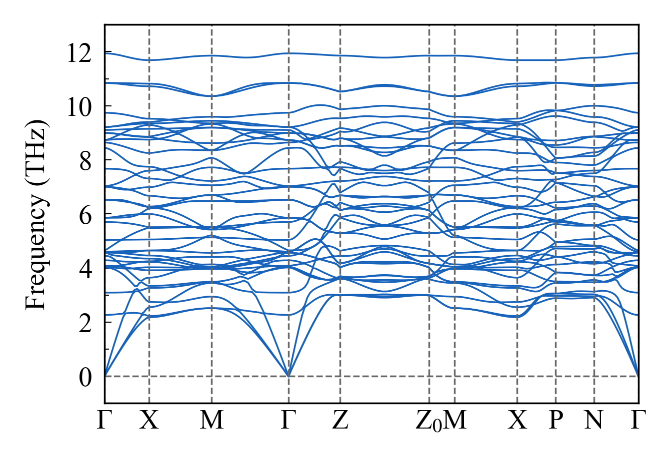
fig.savefig(phonopy_dir/"phonon_band.png", bbox_inches='tight', dpi=1200)提取声子态密度数据
# 绘制DOSfig_dos, ax_dos = plt.subplots(figsize=(cm(7), cm(5)), dpi=500)ax_dos.plot(freq_range, dos, color=color_map[0], linewidth=1)ax_dos.fill_between(freq_range, dos, alpha=0.3, color=color_map[0])
set_ticks(ax_dos, xrange=(-1, 13, 2), yrange=(0, 9, 2))ax_dos.set_xlabel("Frequency (THz)", fontsize=8)ax_dos.set_ylabel("DOS", fontsize=8)ax_dos.axvline(0, color='dimgray', linewidth=0.5, linestyle='--')half_plot_set(ax_dos)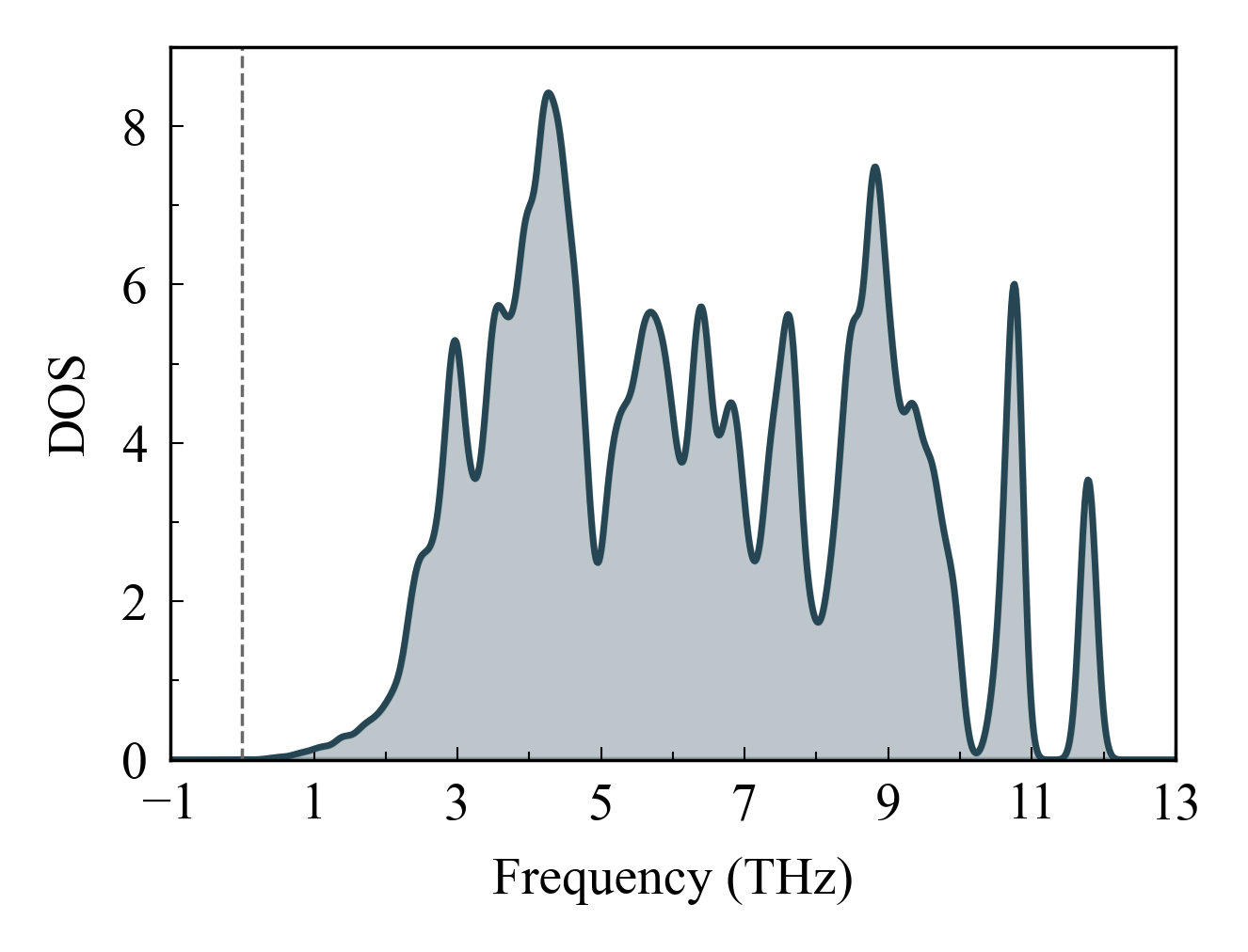
fig.savefig(phonopy_dir/"phonon_DOS.png", bbox_inches='tight', dpi=1200)画一个组合图
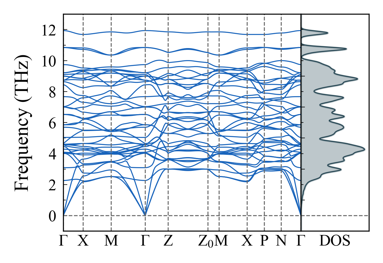
fig.savefig(phonopy_dir/"phonon_band_dos.png", bbox_inches='tight', dpi=1200)